Upregulation
Improvement after certain exposures: hormesis, hypertrophy, and adaptive responses. Large exposures can reverse the benefit.
When does variation help? When does it destroy? A guided journey from nonlinear response curves to evolving ecosystems, risk, control, and cultural memory.
Antifragility is always relative to a system, a source of variation, a measurable payoff, and a defined time window. Improving a response to a particular shock does not imply immunity to all shocks.
E[U(Tω(x))] − U(x) > 0 tests improvement relative to a specified unperturbed baseline. A stronger variability-specific test compares matched distributions with different dispersion and the same mean.
Convexity in a benefit function can favor variation. Convexity in a harm function amplifies fragility. Specify what the vertical axis means.
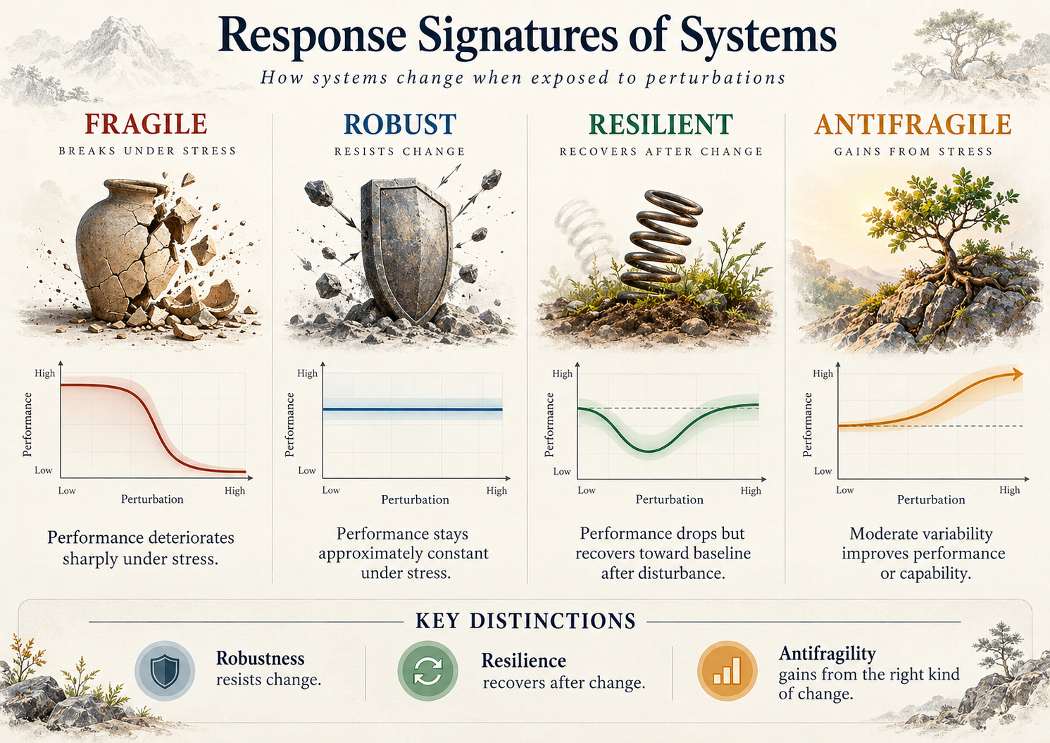
Fragility, robustness, resilience, and antifragility are not interchangeable. The curves illustrate conceptual response signatures; resilience additionally requires a time-dependent recovery description.
Full-resolution image ↗Nassim Nicholas Taleb's foreword, What is Antifragility?, to Applied Antifragility in Natural Systems (2025), organizes apparently disparate phenomena into six classes. The purpose is mathematical transfer between dose-response functions and probability distributions, including the tails.
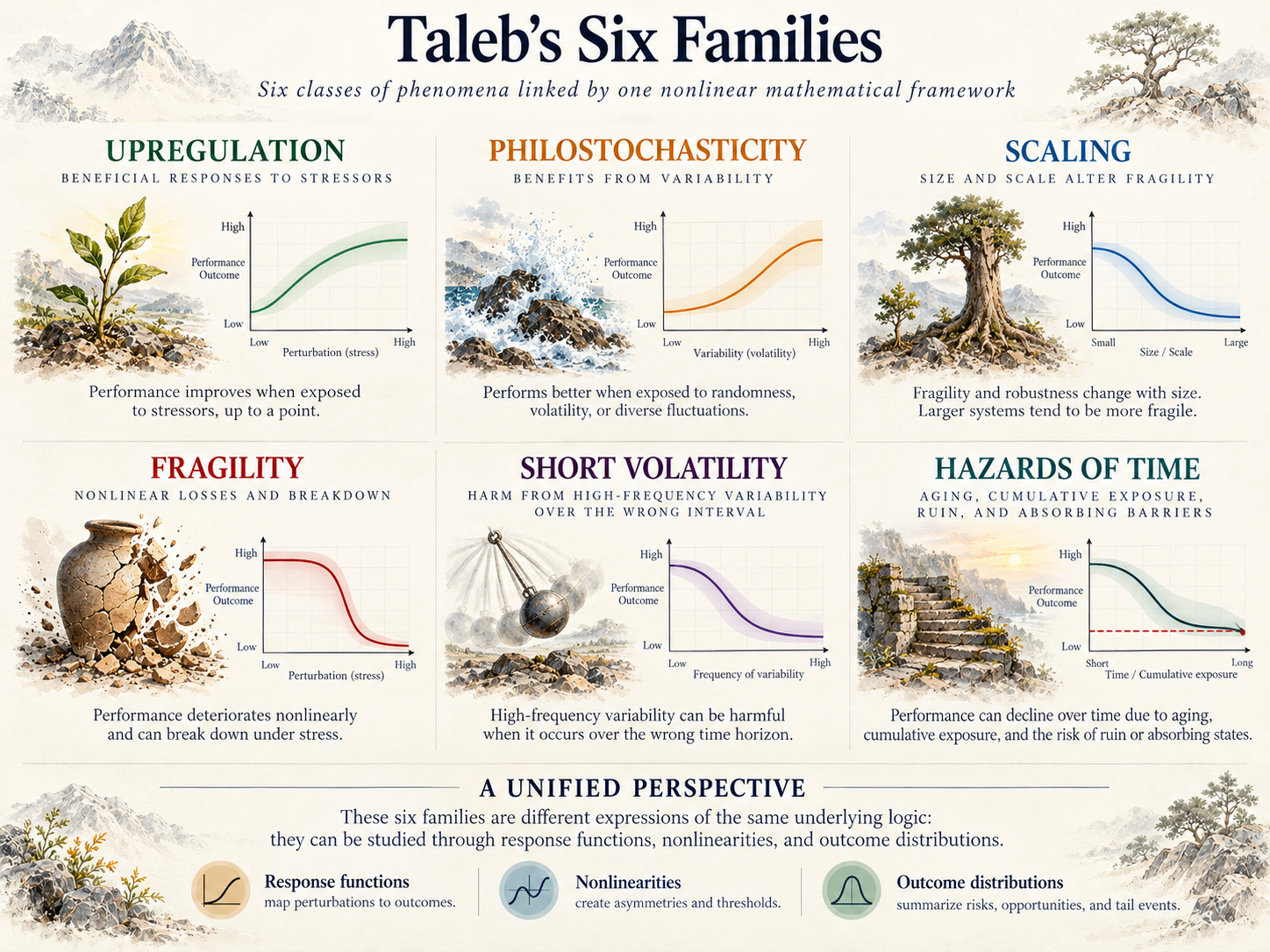
The six classes include both beneficial and harmful responses. They are unified by the analysis of nonlinear functions and outcome distributions, not by a single favorable mechanism.
Full-resolution image ↗Improvement after certain exposures: hormesis, hypertrophy, and adaptive responses. Large exposures can reverse the benefit.
Variability can improve a defined outcome, for example through convex payoffs or variance-sensitive dynamics.
Risk changes with allometry, coupling, and size. Aggregation can create disproportionate failure pathways.
Harm accelerates as shock magnitude grows. A convex loss curve identifies vulnerability to tail outcomes.
The same total exposure can have different consequences when timing, frequency, or recovery intervals change.
Ageing, accumulated risks, and irreversible absorbing barriers change what can survive repeated exposure.
The six labels and their grouping are attributed to Taleb. All explanatory text, diagrams, and models on this website are original paraphrases and synthetic constructions.
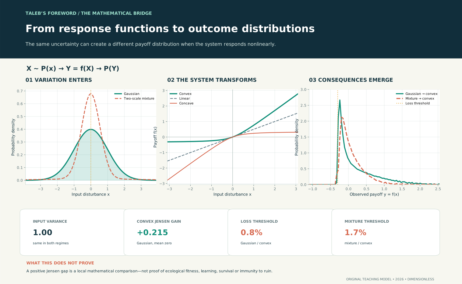
Taleb's foreword is not simply a catalog of six phenomena. Its unifying mathematical idea is that an uncertain input X, passing through a nonlinear response f, becomes a different distribution of consequences Y = f(X). Vary the uncertainty, transform the payoff, and check the entire result—not only its mean.
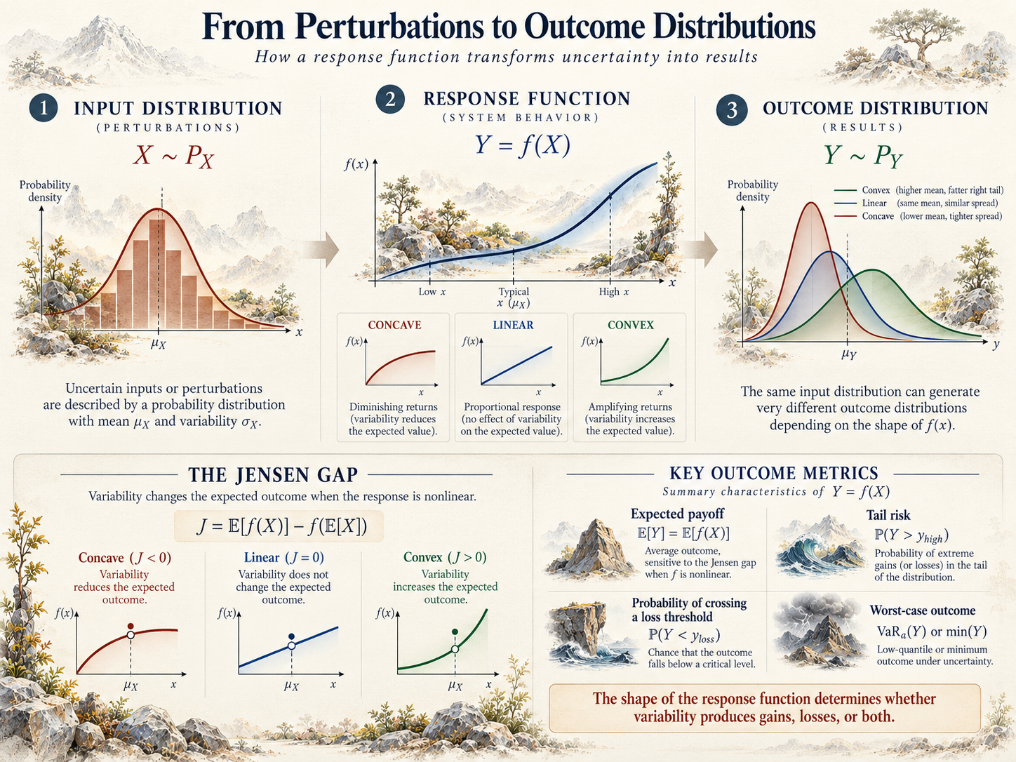
A distribution of inputs is transformed by a response function into an outcome distribution. These plotted distributions are conceptual, not fitted data; the adjacent interactive experiment performs the numerical calculation.
Full-resolution image ↗
Alternative shape with matching mean and population variance.
This is an original synthetic probability model.
Mathematical contract: x is dimensionless; for convex response, f(x) = [x + √(x²+r²) − r]/2. Linear f(x)=x/2; concave f(x)=[x − √(x²+r²) + r]/2. These functions share f(0)=0 and f′(0)=1/2. A positive Jensen gap is not a long-term dynamic improvement, and P(Y≤L) is not a modeled probability of irreversible ruin.
SOURCE: Nassim Nicholas Taleb, “What is Antifragility?”, foreword to Axenie, Bauer, López Corona & West (2025), Applied Antifragility in Natural Systems, Springer, pp. vii–ix. This model, wording and artwork are new educational interpretations, not reproduced figures or a quotation of the foreword.
Each panel illustrates one class from the foreword. The controls change a synthetic model, not observations from natural systems.
Six concepts / six interactive response curves
A stylized response to an input dose.
Moderate stress can enhance a response, while overload can reverse the effect.
Positive response is local; a different outcome or excessive dose may be harmful.
The earlier learning modules on fat-tailed sampling and imperfect ecological rules remain interactive. Both are synthetic and expose crucial limits on naive interpretations of antifragility.
Gaussian and Pareto inputs share a theoretical mean of 3. Heavy tails can still make finite samples less informative. This lab diagnoses statistical uncertainty, not antifragility itself.
A single Monte Carlo batch is not a universal sample-size rule. The Pareto example has a finite mean and infinite variance.
A synthetic resource stock is exposed to shared environmental shocks. Responding to an imperfect signal can protect stocks while sacrificing harvest.
No particular ritual, community or ecosystem is represented. The comparison is conditional on this assumed growth and extraction model.
The Springer volume develops mathematical and dynamical approaches spanning natural responses, evolutionary selection, and closed-loop interventions.
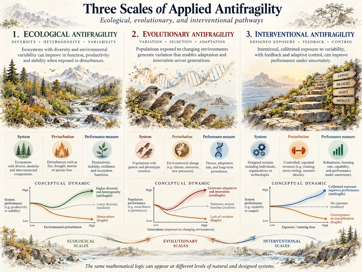
Three research scales illustrate distinct mechanisms and performance criteria. The illustrated trajectories are schematic; beneficial outcomes require system-specific tests.
Full-resolution image ↗Identify benefits from uneven exposure through response-function convexity, where the system and its payoff are explicit.
Examples: dose-response, planetary ecology, neural systems.Study how variation, selection, state transitions, and persistence alter outcomes over multiple generations.
Examples: heterogeneity, adaptive therapy, holobionts.Change the controller or protocol to alter the payoff function while tracking unintended risk and costs.
Examples: tumour-immune-drug dynamics, closed-loop epilepsy control.Four extensions connect applied antifragility with López Corona and collaborators' The Ecology of the Sacred: Constructing an Antifragile Future (author manuscript, 2026). These are frameworks and research directions, not universal empirical findings.
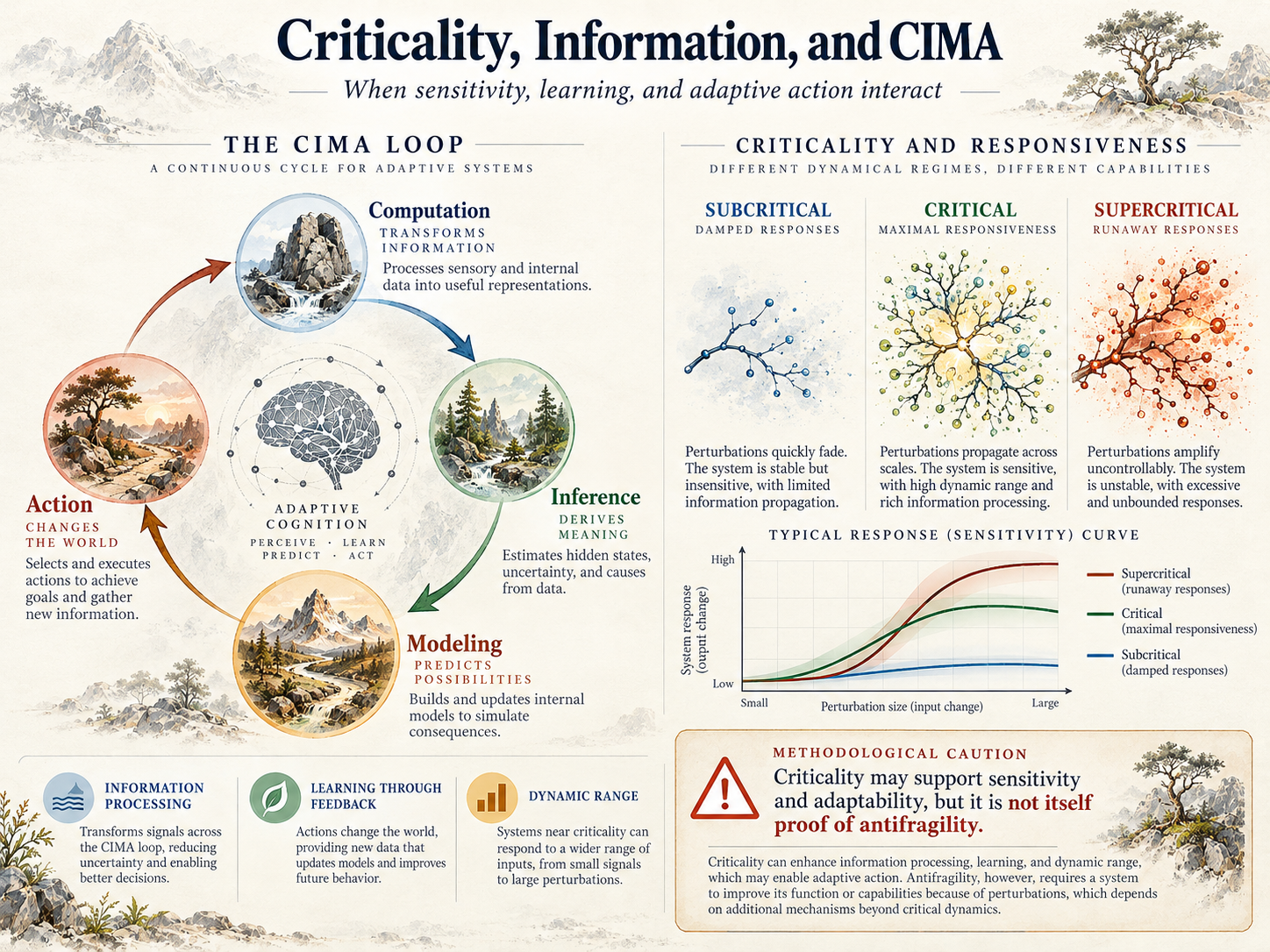
CIMA provides a conceptual information-action cycle. Near-critical dynamics may affect responsiveness, but criticality, high sensitivity, and scale-free patterns do not by themselves establish antifragility.
Full-resolution image ↗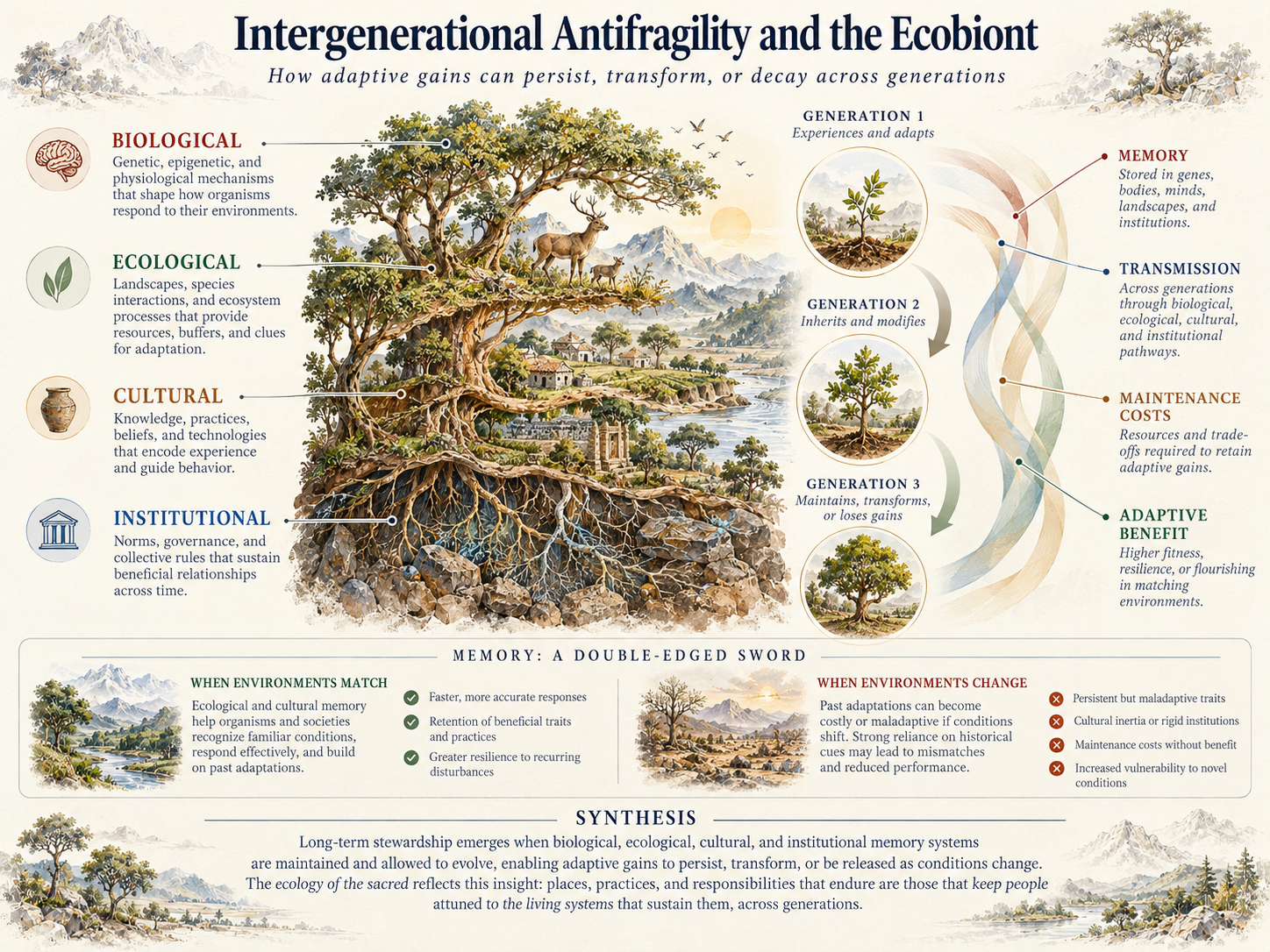
Intergenerational inheritance can preserve, transform, or lose adaptive gains. Memory has maintenance costs and can become maladaptive under environmental change; this plate illustrates a research hypothesis.
Full-resolution image ↗Near-critical organization and information processing may support adaptive response in some systems. Neither spectral 1/f behavior nor criticality is, by itself, an antifragility test.
Compute → Infer → Model → Act. Feedback links ecological signals, representations, action, and the updating of learned behavior.
Genomic, microbial, ecological, and sociocultural channels create different pathways for retaining or losing adaptive capacities.
Calendars, prohibitions, refugia, and ritual obligations can distribute exposure or retain ecological memory. Their effects must be evaluated with local evidence, consent, and attention to historical context.
Six exercises follow the foreword class by class. Eight additional laboratories explore thresholds, adaptive memory, ecological dynamics, fat tails, optionality, risk heuristics, and intergenerational transmission.
For each laboratory, define: the system; input and source of variation; outcome to maximize or loss to minimize; reference; time horizon; costs; and boundary of safe interpretation. Every plotted trajectory is explicitly synthetic. Running a model demonstrates a mechanism under assumed equations, not the presence of that mechanism in observed ecosystems or communities.